Basic information configuration

The first step in model training is to set the basic information, which includes the name, description, problem type, and model architecture.

💡 Tip

A newly generated experiment is named using a timestamp.

Each experiment is created with a system-generated name that includes the creation time and date to ensure uniqueness. While this guarantees traceability, we strongly recommend renaming the experiment to a more descriptive name. For example, based on the dataset, model type, objective, or changed hyperparameters.

Problem type

Each problem type supports specific model architectures with different characteristics. Select the architecture that best fits your use case based on accuracy requirements, inference speed, and computational resources. The platform supports the following problem types and architectures:

Object detection

Object detection identifies and locates multiple objects within an image using bounding boxes. The following architectures can be selected:

Faster R-CNN

Faster R-CNN (Region-based Convolutional Neural Network) is a two-stage detector in which regions are proposed first, then classified, and their bounding boxes are refined.

Paper: arxiv.org/abs/1506.01497

Faster R-CNN architecture. The backbone extracts locally aware patch features from the input image. A Region Proposal Network generates candidate regions with objectness scores. Each proposal is then processed in parallel by a box regression head that refines bounding box coordinates, and a classification network that produces per-class confidence scores.

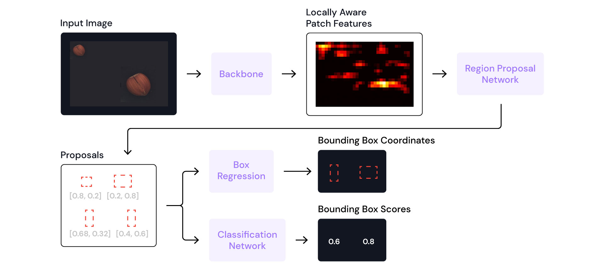
Strengths:

• Accuracy — Given sufficiently large training datasets, it achieves higher accuracy compared to the single-shot detectors.
• Handles small objects well — Better at detecting small or densely packed objects than simpler one-shot detectors.

Weaknesses:

• Limited throughput — Processing is slower than single-shot alternatives like YOLO, resulting in a lower cycle time.
• Heavier model — Uses more memory during inference than lightweight alternatives.

Backbone Options:

Backbone	Description	Speed	Accuracy
MobileNetV3	Lightweight, efficient backbone	Higher	Lower
ResNet50	Deeper backbone for higher accuracy	Lower	Higher

Key Parameters:

• Score threshold (range 0.0 – 1.0, default: 0.05)
  Confidence score below which detections are ignored. The detected bounding boxes can be further filtered out using Polygon Threshold node.

  • Lower values keep more detections, including low-confidence ones. Useful when you don't want to miss any objects, but may include false positives.
  • Higher values reduce false positives but may miss legitimate objects with lower confidence scores.

• NMS threshold (range 0.0 – 1.0, default: 0.5)
  Controls how much bounding box overlap is allowed before boxes are merged.

  • Lower values: Removes more duplicate boxes but may split legitimate overlapping objects.
  • Higher values: Keeps more boxes including overlapping ones. Useful for detecting tightly clustered objects

• Max detections per image
  Maximum number of objects the model can return per image

  • Lower values: Higher processing speed.
  • Higher values: Important for scenes with many objects, but may slow down processing.

Recommended use cases: Counting objects, use cases with lower cycle time. Detecting and classifying multiple objects in a scene.

---

Anomaly detection

Anomaly detection identifies defects or abnormalities in images by learning what "normal" looks like during training. Two architectures are available:

PatchCore

PatchCore is a memory-based anomaly detection method that stores representative patches from normal training images. During inference, it compares test patches against the memory bank to detect anomalies.

Paper: arxiv.org/abs/2106.08265

PatchCore — training phase. Normal training images are passed through a pretrained encoder to extract patch features. These features are reduced via coreset subsampling and stored in a memory bank.

PatchCore — inference phase. Patches are extracted from the input image using the pretrained encoder. The nearest neighbour search compares these patches against the ones in the memory bank to produce an anomaly score and a pixel-level anomaly map highlighting defective regions.

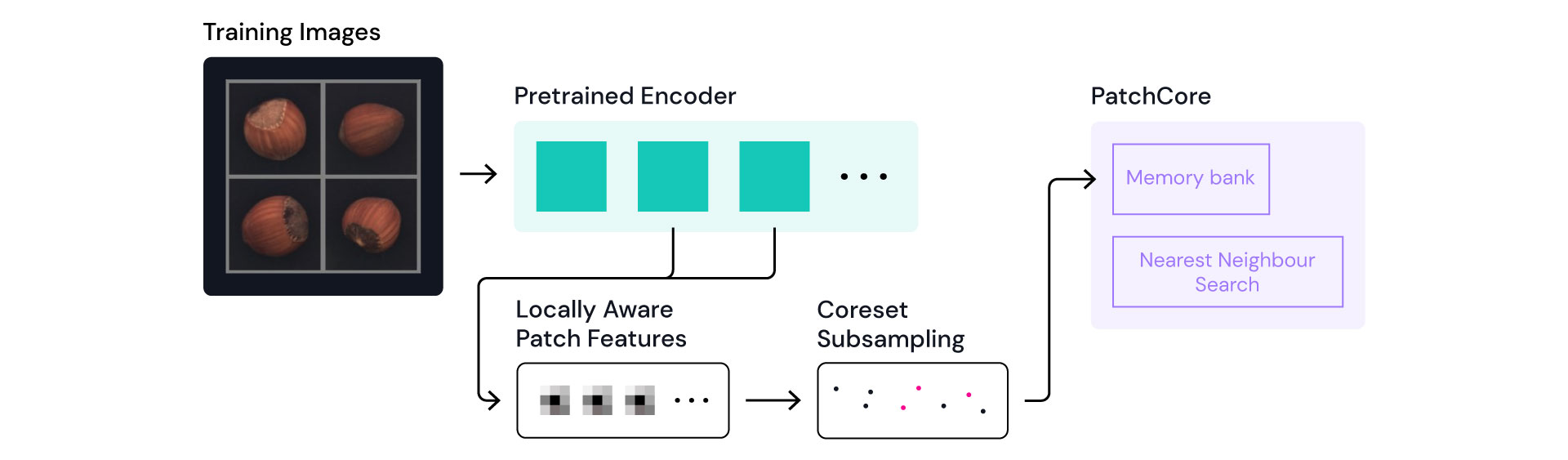
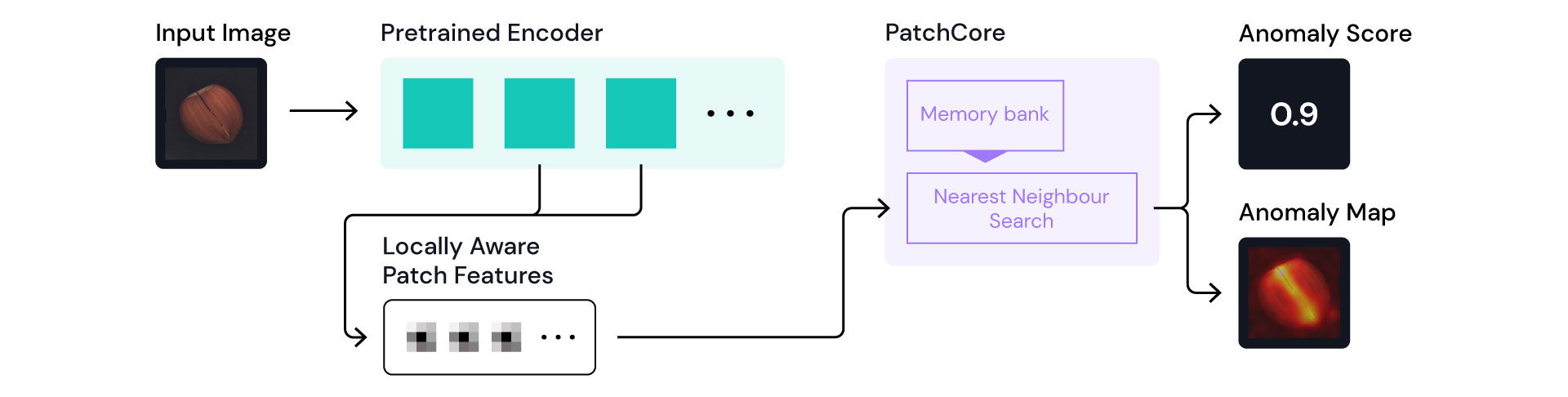
Strengths:

• High localization accuracy — PatchCore can detect small inconsistencies in the image.
• Pinpoints defects — Produces heatmaps showing exactly where anomalies are located in the image.
• Few images needed — Can achieve good results with a relatively small set of reference images.

Weaknesses:

• Memory grows with data — The memory bank can become large with more training images, leading to out-of-memory errors.
• Inference speed — Inference speed slows down with the increasing memory bank (more training images).
• Misses subtle defects — Small surface anomalies like hairline cracks may slip through.
• Data requirements — Training dataset needs to contain a large variation in normal images to reduce false positives.

Backbone Options:

Backbone	Description	Speed	Accuracy
ResNet18	Lightweight backbone, faster training and inference	Fast	Lower
Wide ResNet50-2	Deeper backbone for complex patterns	Slower	Higher

Key Parameters:

• Subsample fraction: Fraction of the memory bank to keep after pruning (reduces memory but may affect accuracy).
• Number of neighbors: Number of nearest neighbours used for classifying the patch.

Recommended use cases: Visual quality inspection with an open set of defects, quality assurance with a limited number of defective samples.

---

FastFlow

FastFlow uses 2D normalizing flows for anomaly detection, learning the probability distribution of normal images. It can detect anomalies by evaluating the likelihood of test images under this learned distribution.

Paper: arxiv.org/abs/2111.07677

FastFlow architecture. A pretrained encoder extracts feature maps from the input image. The FastFlow normalizing-flow modules learn the distribution of normal features and output an anomaly score together with a pixel-level anomaly map.

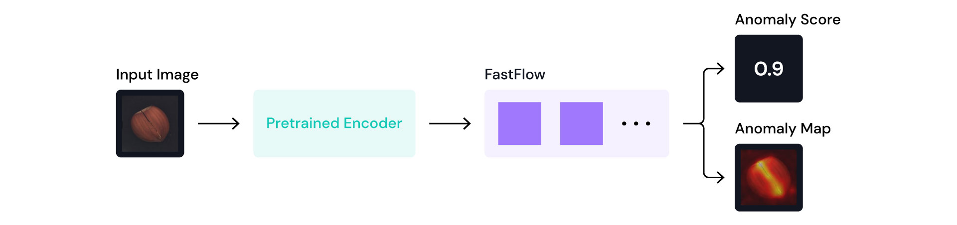
Strengths:

• Fast execution — More efficient than PatchCore; better suited for higher cycle time use cases.
• Scalability — The model can be trained on large datasets without affecting the inference speed.
• Global information — Unlike PatchCore, FastFlow can utilize global information in the image to produce anomaly scores.

Weaknesses:

• Lower localization accuracy — The produced anomaly heatmaps are less accurate than PatchCore.

Backbone Options:

Backbone	Description	Speed	Accuracy
ResNet18	Lightweight backbone, faster training and inference	Fast	Lower
Wide ResNet50-2	Deeper backbone for complex patterns	Slower	Higher

Key Parameters:

• Flow steps: Number of transformation steps (more steps = more complex distributions but higher computation time).
• Hidden ratio: Ratio of hidden layer size to input size. Determines the capacity of the model. Higher value results in a more expressive model, but leads to higher computation time.

Recommended use cases: texture anomaly detection, classifying defective samples from non-defective ones.